Project Overview
Obesity is a complex global health challenge driven by a combination of genetic, environmental, and lifestyle factors. This project aims to build a robust machine learning pipeline to predict an individual's obesity level based strictly on their eating habits and physical condition.
Developed entirely with scikit-learn, the project rigorously compares three foundational algorithms: K-Nearest Neighbors (KNN), Decision Trees, and Support Vector Classifiers (SVC). To maximize predictive power, these models are subsequently combined into a Voting Ensemble. The full implementation and exploratory data analysis can be found in the classification_analysis.ipynb notebook.
The Dataset & SMOTE Balancing
The data originates from the UCI Machine Learning Repository and contains 2,111 records across 16 features.
A critical aspect of this dataset is its class balance strategy. Only 23% of the data was collected directly from users via a web platform. The remaining 77% was synthetically generated using the SMOTE (Synthetic Minority Over-sampling Technique) algorithm. SMOTE works by selecting minority class examples and interpolating new, synthetic data points along the line segments joining them to their $k$ nearest neighbors. This perfectly balances the 7 distinct levels of the NObeyesdad target variable (ranging from Insufficient Weight to Obesity Type III), preventing the models from developing a majority-class bias.
Feature Breakdown
- Demographics & Physical:
Gender,Age,Height,Weight,family_history_with_overweight - Eating Habits:
FAVC(Frequent high-calorie food),FCVC(Vegetables frequency),NCP(Number of main meals),CAEC(Food between meals),CH2O(Daily water). - Physical Condition:
SMOKE,SCC(Calories monitoring),FAF(Physical activity frequency),TUE(Time on tech devices),CALC(Alcohol consumption),MTRANS(Transportation mode).
Data Preprocessing: Scaling & The Dummy Variable Trap
Machine learning models require mathematical transformations to process raw data correctly. This project utilizes a ColumnTransformer to route different data types through specific pipelines:
1. StandardScaler for Numerical Data: Algorithms like KNN and SVC rely on geometric distance metrics (like Euclidean distance). If a feature like Weight ranges from 50 to 150, and Age ranges from 18 to 60, the model will disproportionately weight the larger magnitude. StandardScaler transforms features to have a mean of $0$ and a standard deviation of $1$ ($z = (x - u) / s$), ensuring equal feature contribution.
2. OneHotEncoder & The Dummy Variable Trap: Nominal categorical data (e.g., Gender) cannot be assigned arbitrary integers (1=Male, 2=Female) because algorithms might assume mathematical relationships (2 > 1). OneHotEncoder creates binary columns for each category. However, this causes perfect multicollinearity (if Gender_Female is 0, Gender_Male MUST be 1). To ensure mathematical stability, we use drop="if_binary" (or drop="first"), which drops one redundant column, effectively avoiding the "Dummy Variable Trap".
from sklearn.compose import ColumnTransformer
from sklearn.preprocessing import StandardScaler, OneHotEncoder
from sklearn.pipeline import Pipeline

num_cols = ["Age", "Height", "Weight", "NCP", "CH2O", "FAF", "TUE"]
cat_cols = ["Gender", "family_history_with_overweight", "FAVC", "FCVC", "CAEC", "SMOKE", "SCC", "CALC", "MTRANS"]

# Prevent Data Leakage by embedding transformations inside the pipeline
preprocess = ColumnTransformer([
    ("num", StandardScaler(), num_cols),
    ("cat", OneHotEncoder(handle_unknown="ignore", drop="if_binary"), cat_cols),
])
1. K-Nearest Neighbors (KNN)
Mathematical Intuition: KNN is a non-parametric, instance-based learning algorithm. It does not "learn" a mapping function during training; it memorizes the dataset. During inference, it calculates the distance $d(p, q) = sqrt{sum_{i=1}^{n} (q_i - p_i)^2}$ between the new sample and all existing training samples, assigning the majority class of the $k$ closest neighbors.
Pros: Simple, interpretable, and makes no prior assumptions about data distribution.
Cons: Extremely susceptible to the "Curse of Dimensionality" and computationally expensive at inference time ($O(n times d)$ complexity).
Read more: Nearest neighbor pattern classification (Cover & Hart, 1967)
2. Decision Tree Classifier
Mathematical Intuition: This algorithm recursively partitions the feature space using orthogonal splits. At each node, it selects the feature and threshold that maximizes Information Gain or minimizes Gini Impurity ($Gini = 1 - sum p_i^2$), creating a highly interpretable "white-box" flowchart.
Pros: Handles non-linear relationships naturally, unaffected by unscaled data, and extremely fast at inference.
Cons: High variance; easily overfits the training data (memorizes noise) if parameters like max_depth or min_samples_split are not strictly tuned.
Read more: Classification and Regression Trees (Breiman et al., 1984)
3. Support Vector Classifier (SVC)
Mathematical Intuition: SVC seeks the optimal hyperplane that maximizes the margin between classes. Because lifestyle data is rarely linearly separable, we employ the Kernel Trick, specifically the Radial Basis Function (RBF) kernel: $K(x, x') = exp(-gamma ||x - x'||^2)$. This implicitly maps the features into an infinite-dimensional space where a linear hyperplane can separate the obesity classes.
Pros: Exceptionally powerful in high-dimensional spaces and robust against overfitting.
Cons: Training complexity scales cubically $O(n^3)$, making it drastically slow on large datasets. It also does not compute probabilities natively (requires Platt scaling).
Validation Strategy: LOOCV vs K-Fold
To ensure models generalize well to unseen data, hyperparameter tuning was performed using GridSearchCV.
Two validation strategies were tested: Standard K-Fold Cross Validation and Leave-One-Out Cross Validation (LOOCV). While LOOCV provides an almost unbiased estimate of true performance by training $N$ separate models (one for each data point), it highlighted a severe architectural limitation: SVC became completely unfeasible. Due to SVC's $O(n^3)$ complexity, running 2,111 separate training iterations exhausted practical compute budgets, proving that mathematically heavy models require K-Fold validation in real-world scenarios.
4. Voting Classifier (Ensemble)
Ensemble methods rely on the "wisdom of the crowd" theorem, which dictates that aggregating multiple weak or distinct learners produces a stronger meta-learner with lower variance. The VotingClassifier combines our DT, KNN, and SVC models:
Hard Voting: Uses strict majority rule (mode of the predictions).
Soft Voting: Averages the predicted probability matrices (e.g., Model A says 90% Obese, Model B says 60% Obese = 75% average). It typically yields better results as it respects the "confidence" of each model.
from sklearn.ensemble import VotingClassifier

# Note: SVC must be initialized with probability=True to participate in Soft Voting
voters = [
    ("knn", knn_pipeline),
    ("dt", dt_pipeline),
    ("svc", svc_pipeline)
]

hard_voting = VotingClassifier(estimators=voters, voting="hard")
soft_voting = VotingClassifier(estimators=voters, voting="soft")
Results — Standard K-Fold Validation
| Model | Accuracy | Precision | Recall | F1-Score |
|---|---|---|---|---|
| DecisionTreeClassifier | 0.9409 | 0.9421 | 0.9409 | 0.9411 |
| KNeighborsClassifier | 0.8818 | 0.8806 | 0.8818 | 0.8802 |
| SVC (RBF Kernel) | 0.9598 | 0.9606 | 0.9598 | 0.9597 |
Results — Leave-One-Out Validation (LOOCV)
| Model | Accuracy | Precision | Recall | F1-Score |
|---|---|---|---|---|
| DecisionTreeClassifier | 0.9409 | 0.9425 | 0.9409 | 0.9413 |
| KNeighborsClassifier | 0.8629 | 0.8611 | 0.8629 | 0.8610 |
| SVC | Timeout / Too slow | - | - | - |
Results — Voting Ensembles
| Voting Mode | Accuracy | Precision | Recall | F1-Score |
|---|---|---|---|---|
| Hard Voting | 0.9669 | 0.9671 | 0.9669 | 0.9668 |
| Soft Voting | 0.9716 | 0.9721 | 0.9716 | 0.9715 |
Conclusions & Architectural Takeaways
- The Dominance of Soft Voting: By leveraging the probabilistic confidence of multiple distinct mathematical approaches, the Soft Voting ensemble achieved state-of-the-art performance for this dataset (97.16% Accuracy and 0.97 F1-Score).
- The Computational Cost of Margins: While the Support Vector Classifier (SVC) was the best individual standalone model, the LOOCV experiment proved it is not scalable for rapid iterative training on large datasets without dedicated compute clusters.
- Decision Tree as the Pragmatic Baseline: Despite its simplicity, the Decision Tree provided an impressive 94% accuracy with virtually zero training latency, proving that highly interpretable "white-box" models are often the most pragmatic choice for budget-constrained production environments.